A summary of quick and useful numerical methods to compute a definite integral of the form:

When implementing some tasks we often use unnecessary complex integration methods just because they are available in most scientific computing languages. They are usually more accurate but at the expense of speed. When computational time is important it is worth to know these faster and easy to implement integration methods.
Trapezoidal rule of integration
The trapezoidal rule of integration approximates the function  to be integrated by a first order polynomial
  . If we chose
  and
and  as the two points to approximate by
  we can solve for
  and
and  , leading to
To be more accurate, we usually divide the interval ![{[a, b]}](https://s0.wp.com/latex.php?latex=%7B%5Ba%2C+b%5D%7D&bg=ffffff&fg=000000&s=0&c=20201002) into
into  sub-intervals, such that the width of each sub-interval is
  . In this case, the trapezoidal rule of integration is given by
![\displaystyle I \approx \frac{(b-a)}{2n}\bigg[f(a) + 2\bigg(\sum_{i=1}^{n-1} f(a+ih)\bigg) + f(b)\bigg]](https://s0.wp.com/latex.php?latex=%5Cdisplaystyle+I+%5Capprox+%5Cfrac%7B%28b-a%29%7D%7B2n%7D%5Cbigg%5Bf%28a%29+%2B+2%5Cbigg%28%5Csum_%7Bi%3D1%7D%5E%7Bn-1%7D+f%28a%2Bih%29%5Cbigg%29+%2B+f%28b%29%5Cbigg%5D&bg=ffffff&fg=000000&s=0&c=20201002)
The total error on the multi-segment trapezoidal rule is given by
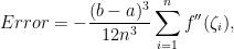
where  is some point in the interval
 ![{[a + (i-1)h, a + ih]}](https://s0.wp.com/latex.php?latex=%7B%5Ba+%2B+%28i-1%29h%2C+a+%2B+ih%5D%7D&bg=ffffff&fg=000000&s=0&c=20201002) .
.
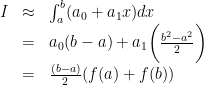
Simpson  rule of integration
The Simpson rule of integration approximates the function to be integrated by a second order polynomial  . If we chose ,
  and as the three points to approximate by
  we can solve for , and
  , leading to
![\displaystyle \begin{array}{rcl} I & \approx & \int_{a}^{b} (a_0 + a_1x + a_2 x^2)dx\\ & = & \frac{h}{3}\bigg[f(a) + 4f\bigg(\frac{a+b}{2}\bigg) + f(b)\bigg] \end{array}](https://s0.wp.com/latex.php?latex=%5Cdisplaystyle+%5Cbegin%7Barray%7D%7Brcl%7D+I+%26+%5Capprox+%26+%5Cint_%7Ba%7D%5E%7Bb%7D+%28a_0+%2B+a_1x+%2B+a_2+x%5E2%29dx%5C%5C+%26+%3D+%26+%5Cfrac%7Bh%7D%7B3%7D%5Cbigg%5Bf%28a%29+%2B+4f%5Cbigg%28%5Cfrac%7Ba%2Bb%7D%7B2%7D%5Cbigg%29+%2B+f%28b%29%5Cbigg%5D+%5Cend%7Barray%7D+&bg=ffffff&fg=000000&s=0&c=20201002)
Again, if we divide the interval into equidistant sub-intervals each of length  , such that
  , and apply the Simpson rule of integration in each sub-interval we get
![\displaystyle I \approx \frac{(b-a)}{3n}\bigg[f(x_0) + 4\sum_{i=1,\ i=\text{odd}}^{n-1} f(x_i) + 2\sum_{i=2,\ i=\text{even}}^{n-2} f(x_i) + f(x_n)\bigg]](https://s0.wp.com/latex.php?latex=%5Cdisplaystyle+I+%5Capprox+%5Cfrac%7B%28b-a%29%7D%7B3n%7D%5Cbigg%5Bf%28x_0%29+%2B+4%5Csum_%7Bi%3D1%2C%5C+i%3D%5Ctext%7Bodd%7D%7D%5E%7Bn-1%7D+f%28x_i%29+%2B+2%5Csum_%7Bi%3D2%2C%5C+i%3D%5Ctext%7Beven%7D%7D%5E%7Bn-2%7D+f%28x_i%29+%2B+f%28x_n%29%5Cbigg%5D&bg=ffffff&fg=000000&s=0&c=20201002)
The total error on the multi-segment Simpson rule is given by

where is some point in the interval ![{[x_{i-1}, x_{i+1}]}](https://s0.wp.com/latex.php?latex=%7B%5Bx_%7Bi-1%7D%2C+x_%7Bi%2B1%7D%5D%7D&bg=ffffff&fg=000000&s=0&c=20201002) .
.
Gaussian quadrature rule of integration
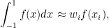
A quadrature rule of integration [2] approximates the integral  by a weighted sum of function values at specified points within the domain of integration,

The Gaussian quadrature rule is constructed to yield an exact result for polynomials of degree  or less by a suitable choice of points
  and weights
  ,
,  .
.
By convention the domain of integration for such a rule is taken as ![{[-1, 1]}](https://s0.wp.com/latex.php?latex=%7B%5B-1%2C+1%5D%7D&bg=ffffff&fg=000000&s=0&c=20201002) ,
,
which means that applying the Gaussian quadrature to solve an integral over takes the following form:

It can be shown that the evaluation points are just the roots of a polynomial belonging to a class of orthogonal polynomials. The approximation above will give accurate results if the function is well approximated by a polynomial of degree  or less. In that case the associated polynomials are known as Legendre polynomials and the method is known as Gauss-Legendre quadrature.
Here we can find the Gauss-Legendre’s quadrature weights and Abscissae values , for different values of .
The total error of the Gauss-Legendre quadrature rule is given by
![\displaystyle \frac{(b-a)^{2n+1}(n!)^4}{(2n+1)[(2n)!]^3} f^{(2n)}(\zeta), \quad a<\zeta<b](https://s0.wp.com/latex.php?latex=%5Cdisplaystyle+%5Cfrac%7B%28b-a%29%5E%7B2n%2B1%7D%28n%21%29%5E4%7D%7B%282n%2B1%29%5B%282n%29%21%5D%5E3%7D+f%5E%7B%282n%29%7D%28%5Czeta%29%2C+%5Cquad+a%3C%5Czeta%3Cb&bg=ffffff&fg=000000&s=0&c=20201002)
Alternative Gaussian quadrature rules
If the integrated function can be written as 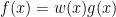 , where
  is approximately polynomial, and
  is known, then there are alternative weights
  such that
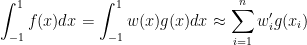
For example, the Gauss-Hermite quadrature rule is used when  .
.
References:
[1] Integration section of the Holistic Numerical Methods website.
[2] Wikipedia page on Gaussian quadrature.
[3] Gauss-Legendre’s quadrature weights and Abscissae values for different values of n.